PID Control

Well, I’m back from another automation training adventure, this time just outside of St. Louis, Missouri. After my previous trip to Denver, I thought it might be a good idea to discuss PID control, since that is what I spent a great deal of time discussing there. The following material is taken directly from my book:

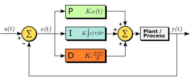
Control of a closed-loop system is often done with PID control algorithms or controllers. A closed-loop system takes feedback from whatever variable is being controlled, such as temperature or speed, and uses it to attempt to maintain a set point. PID stands for proportional-integral-derivative, the names of the variables set in the controlling algorithm. Another name for this is “three-term control.”

In a closed-loop system, a sensor is used to monitor the process variable of the system. This may be the speed of a motor, the pressure or flow of a liquid, the temperature of a process, or any variable that needs to be controlled. This value is then digitized into a numerical value scaled to the engineering units of what is being measured. The variable is then compared to the set point for the system; the difference between the set point and the process variable is the error or difference that must be minimized by the system. This value is “fed back” into the system to counteract the error. The figure at the top of this post shows a graphic diagram of PID control.

For any error that must be compensated for, there is some actuator or value that must be controlled to offset the error. In the case of temperature, this might be a proportional valve that feeds hot water into a system or gas into a burner; for a motor it might be current to increase speed or torque. The current error within the system is closely related to the P or proportional value; in other words, the variable is used as a direct offset to the detected error.

One might think it would be sufficient to simply use the P value to constantly introduce an offset into a process; if one is trying to keep a container of liquid at a constant temperature, why can’t you just add heat until the container is at the desired temperature and then remove the heat? Experience would say that the temperature would either overshoot the set point or take a very long time to get there. There is the possibility that we would want to achieve the set point very quickly, further increasing the overshoot. This is where the other variables, the I and D parameters, are applied.

If the proportional variable is the current error, the integral or I value can be thought of as the accumulation of past errors, while the derivative or D value can be thought of as a prediction of future errors. These values are affected by the rate of change in the sensed PV and, if properly applied, can improve control of the process immensely. The I and D parameters are not always used in the process. One or the other is often omitted, creating the terms PI and PD control.

PID controllers may be a self-contained device such as a panel-mounted temperature controller or an algorithm within a PLC or DCS controlling an analog “loop.” There are various ways to arrive at the P, I, and D values, including the Zeigler-Nichols method, “Good Gain” method, and Skogestad’s method, but one of the most common is the “guess and check” or trial and error method.

Parameters and variables are set in an iterative process after defining the cycle. An example of this process for a temperature loop is illustrated here:

1. Predefine and set up a PV (process variable), CV (control variable), and SP (set point). In this example, assume PV is a temperature input 4 to 20 mA signal (RTD) downstream of the CV, where the CV is a modulating analog steam control valve. The set point would then be the desired water temperature that the PV would need to achieve after steam is added.

2. Set integral and derivative variables to zero (0).

3. Start the process and adjust the proportional/gain tuning parameter until the PV starts modulating above and below the SP.

4. Time a cycle or period of this oscillation. Record this time as the natural period or cycle time.

5. After timing and recording the cycle, reduce the P (proportional) value to half of the setting needed to achieve the natural cycle.

6. At this point set the I (integral) parameter to the natural cycle. This will decrease the amount of time it takes for the PV to reach SP than with the P setting alone.

7. The D (derivative) may generally be safely set to approximately one-eighth of the integral setting. This value helps with “damping” or controlling the overshoot of the process. If a process is noisy or dynamics are fast enough, where PI is sufficient the D value may often be left at 0.

While moving from just the (P) setup to adding the (I) value, it is important to stop and restart the process as well as any setting adjustments that need to be made in a manual mode. If the process remains in automatic and attempts are made to adjust variables, the system will be looking at the previous cycles and will not be a true indication of PID performance in a typical start-up scenario.

There are many other possible modifications to hardware and software PID controllers, such as set point softening, rate before reset, proportional band, reset rate, velocity mode, parallel gains, and P-on-PV. Users should first select the standard PID form when setting up controller values. It is also important to make sure the loop update time is 5 to 10 times faster than the natural period.

Servo systems and software programs usually have auto-tuning algorithms that use results from input information, known system characteristics, and detected loads to approximate PID settings. Many manufacturers preset algorithm variables based on the hardware selected and input information about the process. Process control and servo system loops can act very differently, however, and a general knowledge of PID can be useful in setting initial parameters.